With recent advances in NGS technologies, RNA-seq is now the preferred way to measure gene expression and perform differential gene expression analysis. However, the presence of technical variability can lead to a wrong conclusion as shown by the Sequencing Quality Control (SEQC) project [1], which highlighted the fact that RNA-seq does not accurately measure absolute expression and additionally demonstrated the presence of gene-specific bias. This brings into question the reproducibility and correctness of direct comparison between experiment results. This report will demonstrate the presence of technical bias in several normal tissue RNA-seq experiments and investigate the ability of different normalization methods to address this bias.
1. RNA-seq experiments
Comparing the results of RNA-seq experiments is not such a straightforward job as there are lots of preprocessing steps before diving into experiments comparisons. First of all, estimation of transcript abundance levels can be achieved with either aligning reads or using pseudo-aligning parts of the reads and currently there are more than 10 competing tools for this step. Pseudo-alignment based Kallisto has shown to provide the most consistent and accurate quantifications, yet being computationally cheap as compared to alignment-based algorithms [2]. Secondly, RNA-seq experiments allow scientists to measure transcript abundance (as a proxy for “relative” gene expression as RNA-seq experiment unfortunately cannot measure absolute expression) and can be estimated using different units, such as RPKM (Reads Per Kilobase of exon per Million reads mapped), FPKM (Fragments Per Kilobase of exon per Million fragments mapped) or TPM (Transcripts Per kilobase Million). Among those 3 metrics, TPM seems to be the best way to report RNA-seq gene expression values according to growing amounts of evidence, especially because the sum of TPMs in each sample are the same, making it straightforward to compare abundances between samples [3, 4].
Therefore, for this blog post, gene expression for each experiment has been analysed in terms of transcript abundance using the Kallisto app on Genestack and reported in TPMs (transcripts per kilobase million). Then, normalization and comparison analysis were performed locally in a Jupyter Notebook (code is available here).
In order to dissect the effect of different normalization techniques, we had to carefully choose the RNA-seq experiments so that they can be roughly comparable with each other. In this report we have compared RNA-seq gene expressions from 3 following experiments:
- [E-MTAB-513] Illumina Human Body Map 2.0 Project (GSF099976);
- [PRJEB4337] HPA RNA-seq normal tissues (GSF432860) and
- [GSE30352] The evolution of gene expression levels in mammalian organs (GSF911938).
The experiment data and analysis results are available on the Genestack platform in a folder “RNA-seq re-analysis” (GSF3756545).
Experiment 1: Illumina Human Body Map 2.0 Project – RNA-seq on HiSeq 2000 consisting of 16 human tissue types and 2 replicates per tissue.
Experiment 2: HPA RNA-seq normal tissues – RNA-seq was performed of tissue samples from 95 human individuals representing 27 different tissues in order to determine tissue-specificity of all protein-coding genes.
Experiment 3: The evolution of gene expression levels in mammalian organs – RNA-seq on Illumina Genome Analyser IIx for 10 species and 6 tissue types, both female/male with 2-3 replicates per tissue.
2. Normalization methods for RNA-seq dataIn RNA-seq experiments, technical bias can originate from different sources such as variable sequencing depth, variable transcript abundance level, read mapping uncertainty, sequence base composition and so on [5]. Therefore, the choice of normalization technique can have a huge impact on the results of differential gene expression analysis. In this report I will consider the following normalization techniques:
-
TPMs [6] (Transcripts per million) where counts are normalized by the length of the feature. This is one of the default outputs of Kallisto.
-
Z-score: calculated by subtracting the overall average gene abundance from the raw expression for each gene, and dividing that result by the standard deviation (SD) of all of the measured counts across all samples.
-
Quantile normalization [7]: originally used for microarray normalization under the name of Robust Multichip Average (RMA). The general idea is to make the distribution of counts for each sample in the experiment to look similar.
-
Rank transformation: a straightforward ranking of genes by abundance for each sample.
-
YuGene [8] normalization: uses the cumulative proportion transform. For each sample, the YuGene score of each gene is proportional to the cumulative sum of the expressions of all the genes with a smaller expression value than the current one.
-
Effective Fold [9] transformation: corresponds to expression level relative to the sample average and make it centred around zero.
-
Adapted Sigmoid function [10] (our own developed method), a special case of logistic function also known as hyperbolic tangent, applied to the data normalized by 99.9 percentile. This function is commonly used in neural networks as activation function and scale the data to [0, 1] range. The following equation was used (where x is expression values and P99.9 is 99.9 percentile):

3. Results
Using raw TPM counts, the first experiment (not taking into account 16 mixed tissues) shows good concordance between gene abundance levels of within-tissue replicates, where the average Pearson's correlation of each tissue’s replicates was around 94%. However, correlation for each sample with all other tissues was much lower at around 67%. This is illustrated by the heatmap below:
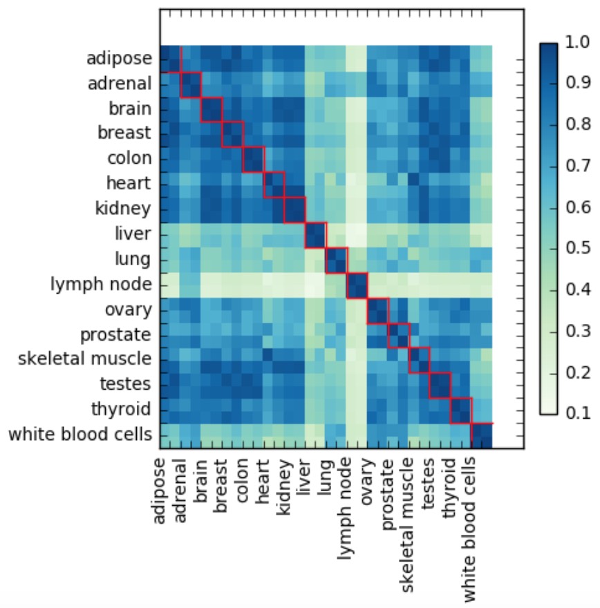
Each value in the heatmap is a Pearson's correlation coefficient and red squares indicate replicates originating from the same tissue (in this experiment each tissue had 2 replicates).
The results of normalization on average correlation within- and between- tissue samples in each experiment is shown below. The first value corresponds to the correlation between replicates for each tissue and the second value represents correlation across different tissues. Ideally, we want the first value to be as high as possible (close to 1) and the second value to be as low as possible (close to 0).
| Method/Experiment | Experiment 1 | Experiment 2 | Experiment 3 |
| EF (effective fold) | 0.990/0.834 | 0.970/0.830 | 0.949/0.782 |
| YuGene | 0.988/0.798 | 0.962/0.769 | 0.937/0.724 |
| Sigmoid | 0.980/0.741 | 0.950/0.685 | 0.914/0.653 |
| Rank transformation | 0.955/0.867 | 0.966/0.879 | 0.916/0.843 |
| Z-score | 0.943/0.674 | 0.899/0.486 | 0.884/0.737 |
| Raw data | 0.943/0.674 | 0.899/0.486 | 0.884/0.737 |
| Quantile normalization | 0.926/0.686 | 0.896/0.518 | 0.890/0.742 |
This table can be visualized as scatter plot as shown below. Each dot represents average correlation for each experiment for each normalization methods, and x-axis depicts within-tissue correlation while y-axis shows between-tissue correlation. Lines connect correlation values for the same experiment. Dots for z-score normalization were shown as triangles as applying this method results in the same correlation values as for raw “TPM” counts and therefore overlay and mask blue dots.

Again, we would ideally want correlation to fall as close to the right (high within-tissue correlation) and as low (small between-tissue correlation) as possible. Looking at this scatter plot, it looks like the “sigmoid” method performs the best among all normalization methods, producing higher within-tissue correlation and lower between-tissue correlation (as compared to other normalization methods) for each experiment.
Now, taking into account all three experiments, we have identified that there were 5 common tissues: brain, heart, kidney, liver, testis. Similarly, for each tissue in an experiment, the gene expression was taken as an average gene expression for all the replicates available for that particular tissue.
Average within-tissue Pearson's correlation across all three experiments for TPM counts was ~86%.
The correlations between-experiments for each normalization method are shown below:
| Method | Correlation between experiments for the same tissue | Correlation between experiments for the different tissues |
| Raw data (TPM) | 0.857 | 0.692 |
| Effective Fold | 0.943 | 0.748 |
| YuGene | 0.928 | 0.681 |
| Sigmoid | 0.913 | 0.593 |
| Rank | 0.949 | 0.858 |
| Quantile | 0.840 | 0.690 |
| Z-score | 0.863 | 0.696 |
4. Conclusion
Based on the three experiments shown above, we have seen quite good concordance between "unadjusted" TPM counts for samples within each tissue, namely 86%. However, correlation between different tissues was also quite high (69%). Applying normalization method increases significantly the correlation within tissues, up to almost 95%, but additionally increases the correlation between samples from different tissues, meaning that the application of normalization makes gene expression in each experiment less tissue-specific. Out of the 5 considered normalization methods, our own developed normalization method “Sigmoid” has shown the best performance in terms of improving within-tissue correlation and even lowering between-tissue correlation.
In conclusion, the choice whether to perform the normalization and which method to use relies on the quality of experimental data and the goals to be achieved. It has to be taken into account that most of the normalization methods (especially in the case of rank transformation and Effective Fold method) not only improve the correlation within tissues but also boosts correlation between tissues.
-
SEQC/MAQC-III Consortium, S. (2014). A comprehensive assessment of RNA-seq accuracy, reproducibility and information content by the Sequencing Quality Control Consortium. Nature Biotechnology, 32(9), 903–14.
-
Sahraeian, S. M. E., Mohiyuddin, M., Sebra, R., Tilgner, H., Afshar, P. T., Au, K. F., … Lam, H. Y. K. (2017). Gaining comprehensive biological insight into the transcriptome by performing a broad-spectrum RNA-seq analysis. Nature Communications, 8(1), 59.
-
Conesa, A., Madrigal, P., Tarazona, S., Gomez-Cabrero, D., Cervera, A., McPherson, A., Mortazavi, A. (2016). A survey of best practices for RNA-seq data analysis. Genome Biology, 17(1), 13.
-
Wagner, G. P., Kin, K., & Lynch, V. J. (2012). Measurement of mRNA abundance using RNA-seq data: RPKM measure is inconsistent among samples. Theory in Biosciences, 131(4), 281–285.
-
Zheng, W., Chung, L. M., & Zhao, H. (2011). Bias detection and correction in RNA-Sequencing data. BMC Bioinformatics, 12, 290. https://doi.org/10.1186/1471-2105-12-290
-
Li, B., & Dewey, C. N. (2011). RSEM: accurate transcript quantification from RNA-Seq data with or without a reference genome. BMC Bioinformatics, 12(1), 323.
-
Bolstad, B. M., Irizarry, R. A., Astrand, M., & Speed, T. P. (2003). A comparison of normalization methods for high density oligonucleotide array data based on variance and bias. BIOINFORMATICS, 19(2), 185–193.
-
Lê Cao, K.-A., Rohart, F., McHugh, L., Korn, O., & Wells, C. A. (2014).YuGene: A simple approach to scale gene expression data derived from different platforms for integrated analyses. Genomics, 103(4), 239–251.
-
Williams, G. (2012). A searchable cross-platform gene expression database reveals connections between drug treatments and disease. BMC Genomics, 13, 12.
-
Glaros, A. (n.d.). Data-driven definition of cell types based on single-cell gene expression data. Retrieved from http://www.diva-portal.org/smash/get/diva2:942241/FULLTEXT01.pdf